AMOC for Smarties - atlas - a transatlantic assessment and deep-water ecosystem-based spatial management plan for Europe

Perhaps the most well-known of these models is the ocean conveyor belt in the image above. This vastly simplified schematic of the global circulation shows us the most fundamental view of the Atlantic overturning circulation, with warm water near the surface travelling northwards, only to be cooled in the Labrador and Nordic Seas where it sinks - due to an increase in density - and flows back southwards. The difference in temperature between these northward and southward flows results in a strong northward heat transport, one of the most important climatic aspects of the AMOC. A similar way of looking at the AMOC is in two dimensions. By integrating the ocean currents from east to west across the Atlantic, we arrive at Figure 2 below, which also shows shallow water flowing north and deep water flowing south. This time, we can see that water flows north mainly above 1000 m, and southwards below.

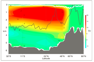
Mean AMOC Stream Function. Credit Buckley and Marshall 2016

Fig. 2. Mean AMOC stream function from Buckley and Marshall (2016). Water flows clockwise around the red area along the colour contours. The stream function, in units of 10⁶m³s^-1 (Sv), is obtained by integrating the total flow in the Atlantic both from east to west, and from top to bottom: i.e. at 24^oN and above 1000 m, about 20 Sv of water flows northwards. The maximum stream function is also called the AMOC index. Grey shading indicates the ocean bottom, and the black line is the crest of the Mid-Atlantic Ridge.

This way of looking at the circulation can also tell us its total strength (i.e. the volume of water flowing northwards in the upper Atlantic per unit time). This is the most commonly used index when attempting to correlate the AMOC with other climate processes, and it is used to say how much the AMOC will weaken in the future. However, this index hides much of the complexity of the system. For example, the overturning can have different strengths at different latitudes. These ideas also tell us little about what the circulation is like in 3D. To better understand the AMOC, we need to think about all the different components that comprise it, and what ultimately drives them.

For a long time, the AMOC - whose name is purely descriptive - was referred to as the ‘Thermohaline Circulation’, a name that implies a driver: heat and salt. This name was used because changes in temperature and salinity affect ocean density, and therefore the ability of water to sink at high latitudes. However, we also know that in the absence of any physical mixing, an ocean driven only by surface heat and salt fluxes will tend to stagnation. The energy required to keep the flow going is actually supplied by winds and tides, and so the term Thermohaline Circulation has fallen out of favour. We must consider the AMOC as both a mechanically- (wind/tide) and buoyancy-controlled system.

Wind directly drives the ocean gyres, a major component of the AMOC. At 26.5 ^oN, where we currently monitor the AMOC in the context of the subtropical gyre, almost all the shallow northward flow is confined within the Gulf Stream. Much of the rest of the upper water column in the gyre actually flows slowly southward, which the 2D view in Figure 2 hides rather neatly. The deeper return flow of the AMOC is partly confined to a western boundary current (again due to gyre circulation), but there are also important pathways in the basin interior, and not all of the water below 1000 m flows southwards. In the subpolar regions the flows become even more complex. The North Atlantic current, a meandering, filamentous boundary between the subtropical and subpolar gyres, becomes the main pathway for northward flow, ultimately feeding warm thermocline water into the Nordic Seas and the Labrador Sea. In the deep ocean, waters spilling over undersea ridges from the Nordic Seas in density-driven currents called ‘overflows’ are important features of the mean circulation. A similar overflow water enters the eastern Atlantic from the Mediterranean, where naturally it then becomes part of the AMOC.

The links between overall AMOC strength and the dynamics of each of its different components are not straightforward. For example, an AMOC slowdown could be driven by changes in wind-forced gyre circulation (often on inter-annual timescales), or by buoyancy-driven changes (decadal or centennial timescales) in Labrador Sea convection, or by convection in the Nordic Seas, or all of the above. At other times, we might get counteracting changes in the deep-water formation regions, which involve very significant changes to local oceanography, but little overall change in AMOC strength. In the presence of a coherent forcing, such as warming and freshening at high latitudes driven by anthropogenic CO₂ emissions, we expect (and are starting to detect) the AMOC to get weaker. But we have yet to fully understand how this thermohaline weakening will interact with each part of the AMOC system, and therefore how it might affect heat transport, carbon cycling and ecosystems.

By: Peter Spooner, ATLAS partner, UCL